


Introduction
Schistosomiasis (also known as Bilharzia) is a chronic disease caused by parasitic worms. Its intestinal form is responsible for severe liver and intestinal damage, physical growth retardation, and cognition and memory problems. The World Health Organization (WHO) reports that more than 200 million people are infected worldwide and an estimated 700 million people are at risk of infection because of their residence in tropical and subtropical areas, and in poor communities without access to safe drinking water and adequate sanitation. Young children are especially vulnerable to infection because of their hygiene and play habits, and the symptoms are quite harmful to them, impairing learning ability and physical development, and even sometimes causing death.
The current who strategy for schistosomiasis control focuses on reducing disease through periodic, targeted treatment with praziquantel. The WHO guidelines identify three strategies based on community prevalence of infection: 1) in communities with a high prevalence (more than 50% infected, we call the high group) universal treatment is conducted once a year; 2) in communities with a moderate prevalence (more than 20% infected but < 50%, we call the moderate group) school-age children are treated once every 2 years; and 3) in communities with a low prevalence (< 20% infected, we call the low group) chemotherapy should be available in health facilities for treatment of suspected cases.1 To implement the WHO strategy, we must effectively classify each community into one of these three categories. A strategy for achieving this aim is the subject of this work.
True prevalence of active infection is defined as the proportion of individuals with at least one worm-pair (one male and one female, otherwise if only one gender is present, they cannot reproduce). Most control programs are based on the detection of eggs by fecal smears on 47 mg slides using the Kato-Katz technique. The observed prevalence is defined as the proportion of individuals who show at least one positive egg count.2 In contrast, the observed prevalence is dependent on the quantity of stool examined in the sample, the number of samples collected (and at which time intervals), and the average worm load (indirectly measured by intensity—eggs/g feces). This is caused by the possibility that a person has worms but that eggs are not present in the stool on a given day, or the eggs are present in the stool, but not in the smear taken from the sample and placed on the slide, or the eggs are on the slide but not seen by the reader. Thus, one has to be careful when designing policy based on observed prevalence. To be concrete, and motivated by the interest in the propagation of the infection, we focus on prevalence as the percentage of individuals with at least one worm-pair. In this way, we can compare prevalence estimates using different algorithms by adjusting the observed prevalence appropriately. Population-level treatment and control are dependent on the measurement of prevalence, thus it is important to investigate the ways of making the measurement as accurately as one can within a reasonable budget, and that is the goal of this work.
Current WHO recommendations for estimating prevalence are based on sample surveys of 50 children/school within the defined ecological zones1; this sample size was possibly selected because it was considered to be the number of sample slides that a survey team examines in a single day. Such an approach typically involves a survey team of several staff moving with a single vehicle, and necessitates entry and analysis of survey data. It is therefore often considered prohibitively expensive for a national program to sustain parasitological surveys on a large scale when this approach is used.3
To reduce screening costs by reducing the number of slides examined, but at the same time not sacrificing any accuracy, we propose a new way to measure prevalence of schistosomiasis that we call pooled testing. The current standard, against which we contrast our proposed method, we call individualed, and it examines 47 mg of feces per slide, taken as four snips from one child's fecal sample smeared on a slide. The pooled method combines snips, of about 12 mg each, from separate fecal samples from four children smeared on a single slide. Both techniques have an observed prevalence that will underestimate the true prevalence (based on the worm-pair definition). Thus, we need to adjust either estimate (the individualed or the pooled) upward to overcome the bias and come closer to the true prevalence.
Previous literature on pooling methods discusses the varying sensitivity of the pooled test with the number of positive samples within a pool. This is known as the “dilution effect.”4 Our model takes into account both the dilution effect and the varying sensitivity of the test with intensity of infection, as modeled by the DeVlas model introduced in the next section.
The model.
The goal of this work is to estimate the true prevalence, the proportion of individuals with at least one worm-pair. The data consist of positive (eggs found) or negative (eggs not found) readings of fecal smear slides, however the slides are constituted. We need to understand the relationship between the true prevalence and probability that eggs are found in the laboratory testing procedure (the sensitivity). Thus, it is necessary to model how the number of eggs per fecal sample varies from person to person and from day to day.
To this end, let P(Y = y; h0x, r) be the probability of finding y eggs in a stool smear (∼12 mg of fecal matter) from a person with x worm-pairs. Let h0 be the number of eggs per smear per worm-pair. Note that the distribution of Y incorporates the variability in egg output in the stool, the variability in the number of eggs captured in the smear, and the variability in what the laboratory technician can actually count. DeVlas considers the negative binomial model where Y ∼ NegBin(h0x, r) with mean h0x and index of aggregation r,5 because r (the index of aggregation in the distribution of egg counts) increases, the variance decreases. The parameter r can also account for imprecision in the measurement of 12 mg of fecal matter per smear. For example, if one smear is actually 16 mg, and another is 8 mg, the difference in egg counts from smear to smear is more variable, which can be built into the model with a smaller value for r. We see below in simulations that the relative benefit of pooling (compared with the individualed method) does not seem to be sensitive to the value of r.
If nm and nf represent the number of male and female worms, respectively, (n = nm + nf) then x = min(nm, nf) is the number of worm-pairs. DeVlas considers nm and nf ∼ Bin(n, 1/2). Let P(X = x∣N = n) be the probability of having x worm-pairs for an individual with worm load n. Let P(N = n; M, k) be the probability of having n worms. Let N ∼ NegBin(M, k) have mean M and index of aggregation k. As k (the index of aggregation in the distribution of worms in the population) increases, the variance decreases. Small values of k indicate more aggregation and relative overdispersion, with the worm counts highly concentrated in a small section of the population. This situation arises in populations with a low level of immunity, where variation in exposure is not countered by the development of immunity. Such low levels of immunity are seen in younger age groups, where there are lower values of k5; another reason there could be a high level of overdispersion in worm load (i.e., a low value for k) would be community variation in exposure to infection. Such heterogeneity could arise from a community being composed of a variety of occupations.5 Thus, when modeling the value of k in a community; one should consider age and homogeneity of exposure. If one chooses to perform Bayesian inference (rather than maximum likelihood), one might then have a prior distribution on k and the prevalence p, which together can be used to compute a prior distribution for M (because prevalence p is a function of k and M). We explore this Bayesian formulation further in Reference 6. The overall distribution of the number of eggs per smear (y) is P(Y = y; M, k, h0, r) (see the Appendix in Reference 5).
Let c be the number of smears per slide. In the literature, c is referred to as the composite sample size, or the pool size. We focus on the case of c = 4 because of common field practice, but our derivations are kept general and our simulation program can accommodate other values of c. To describe collecting c = 4 smears from 1 person on the same day we refer to h0 as the number of eggs per smear per worm-pair, so h = ch0 is the number of eggs per slide (i.e., sample) per worm-pair. We define prevalence as the probability of having at least one worm-pair, so p = P[X > 0] (see Reference 7, Box 1.) We define the c-smear sensitivity as the sensitivity when using c smears from the same individual. See Appendix for mathematical details to derive an expression for sensc, the c-smear sensitivity.
Individualed Prevalence Estimator


For values of the parameters we are investigating, 

Pooled Prevalence Estimator


Although it is possible that 1 − (1 − W)1/c > sens1, for likely values of model parameters, it is a very unlikely event. It will be obvious we are in this unlikely case if our prevalence estimate is greater than 1. Thus, we focus on the estimator 
Bias and bias correction.
Recall that c is the number of smears per slide. In the pooled method we propose, we can consider a slide to be a pool, as in the literature (see References 8–11 for more about pooled testing). Note that our setting differs from the settings in the literature, which either uses a prefect test or a test whose sensitivity does not get diluted in a pool, which is a more realistic model in our setting of testing for estimation of schistosomiasis prevalence.
Let Pc be the probability of a positive slide in the pooled case. With a perfect test, a slide is negative if and only if all c individuals are not infected, therefore 1 − Pc = (1 − p)c, or p = 1 − (1 − Pc)1/c. The quantity H(Pc) = 1 − (1 − Pc)1/c is called the prevalence transformation.8 It takes the probability of a positive pool and transforms it to the probability of a positive individual. Because we are assuming a test with imperfect sensitivity (i.e., sens1 < 1), we denote the prevalence transformation in our case (with Pc given by Eq. [3]) by 


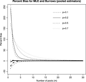
Percent Bias in the mle (

Citation: The American Society of Tropical Medicine and Hygiene 87, 5; 10.4269/ajtmh.2012.12-0216
Key point.
The maximum likelihood estimator (mle) overestimates the prevalence; therefore, we use the Burrows estimator (a type of so-called “shrinking estimator”) that shrinks the estimate slightly, to reduce the bias of our estimator.
Asymptotic mse ratio of the estimators.


We plot this asymptotic mse ratio, as a function of the prevalence p, for c = 4, and for three different values for the sensitivities, sens4 and sens1 (see Figure 2). We choose values to show the case of a perfect test, values from the literature,12 which found that “the overall sensitivity of a single Kato-Katz smear was 70.8%, and it increased with each additional slide to reach 91.7% on examining four smears,” and finally, values to indicate a lower range of sensitivity, because our technique uses less fecal matter than12 to fit all smears onto a single slide. Of importance, the sensitivities from Reference 12 were based on a single stool sample, so the relative change in sensitivity when increasing to four times the fecal matter can be expected to be similar. Increasing the number of stool samples across time has been found to increase the sensitivity more drastically.13 Figure 2 shows that the mse of the pooled estimator is roughly half that of the individualed estimator at prevalences below roughly 30%. This is of interest because we can read half as many slides to achieve the same accuracy of prevalence estimation. Note that we are in some sense making an unfair comparison because the slides from the pooling technique use fecal matter from more individuals. However, the comparison is the comparison of interest because the cost is dominated by the cost of slides and the cost of reading each slide not on the amount of fecal matter used.
MSE ratio pooled to individualed: For three example settings of the sens4 and sens1.
Citation: The American Society of Tropical Medicine and Hygiene 87, 5; 10.4269/ajtmh.2012.12-0216
Note also that with a perfect test, below prevalences of roughly 50%, the pooled estimator has smaller asymptotic mse than the individualed estimator. The poor performance of a pooled estimator at high prevalences has been well studied (see References 8–11) and results from the fact that getting all positive pools is not informative. Note however, this upper bound gets higher as the sensitivities decrease, because lower sensitivity lowers the probability of all positive pools.
Intuitively, the four smears from the same individual may be redundant, because egg counts per smear are positively correlated.† The DeVlas model described previously accounts for this because of the correlation of egg counts within an infected individual. Thus, in general, sens4 < 1 − (1 − sens1)4. This holds for the observed sensitivities in Reference 12 where 0.917 < 1 − (1 − 0.708)4 = 0.993 and more extremely for 0.6 < 1 − (1 − 0.4)4 = 0.8704, our third example of sensitivities. We see in Figure 3 that this property of the sensitivities pushes the curve downward, making pooling more efficient relative to not pooling. Furthermore, as sens1 gets closer and closer to sens4, we get closer and closer to the usual pooling setting in which it is assumed that sensitivity does not decrease with pooling. In other words, having only one infected smear on a slide is just as easily detected as having four infected smears. This is likely not true in general for schistosomiasis, but may be close to true in situations of a high intensity of infection, when infected people have many worms, which therefore produce many eggs. This is likely to hold true in regions where there has been no treatment available for a long time, so infections have been allowed to grow stronger and worms have multiplied enormously. Thus, assuming constant and known values for sens1 and sens4 for the population, we see from the previous derivation that pooling is much more efficient, allowing for reading half the slides to achieve the same level of accuracy.
MSE ratio pooled to individualed: Comparing sens4 < 1 − (1 − sens1)4 to sens4 = 1 − (1 − sens1)4.
Citation: The American Society of Tropical Medicine and Hygiene 87, 5; 10.4269/ajtmh.2012.12-0216
In Figure 4, we examine the effect of decreasing to a pool size of c = 2. We obtain values for sens1, sens2, sens4 by the DeVlas model with parameters M = 500, k = 0.2, h0 = 0.085, r = 1.6, and plot the ratio of pooled/individualed mse for a pool size of two and four. We see that a pool size of two is less beneficial for lower prevalences, but does slightly better at higher prevalences (above roughly 50%). Because we are most likely dealing with prevalences below 50% (and those above 50% are all treated the same according to the WHO recommendations), we decided to proceed with the pool size of four. Beyond four is likely infeasible as a laboratory procedure.
MSE ratio pooled to individualed: Comparing c = 4 to c = 2 for sens4 = 0.88, sens2 = 0.83, and sens1 = 0.76.
Citation: The American Society of Tropical Medicine and Hygiene 87, 5; 10.4269/ajtmh.2012.12-0216
Figure 2 assumes constant values for sens4 and sens1, which are known and chosen correctly in the estimators. In reality however, they depend on the parameters M, k, h0, r. Because we do not know the parameter values, we do not know the true values of sens4 and sens1 or the true prevalence. Because prevalence is a function of M and k, the values for sens4 and sens1 will change with the prevalence. The asymptotic expression for mse above does not incorporate this added complexity. To get a picture of how the mse ratio behaves with a finite number of slides (we use the current standard of m = 50 slides) and to explore how the mse ratio is affected by varying the parameters M, k, h0, r in the model, we turn to simulations.
Key point.
The mean square error of an estimator measures the square of the average amount by which the estimator misses the quantity we are trying to estimate (for us, the prevalence). It plays the role of the variance when dealing with a biased estimator. By asymptotic, we mean we examine this error as the sample size approaches infinity. We compare the pooled and individualed estimators by their asymptotic mean square error to see which one does better at estimating prevalence as the sample size approaches infinity. Figure 2 shows us that the mean square error of the pooled estimator is roughly half that of the individualed estimator at prevalences below roughly 30%. This is of interest because we can read half as many slides to achieve the same accuracy of prevalence estimation.
Simulations
For each plot, we fix three of the four parameters M, k, h0, and r and vary the fourth parameter to study the variance, bias, and mse change for the pooled and individualed estimators. In contrast to the asymptotic analysis, we now allow the true sensitivities to vary with the varying parameter values. In other words, for the individualed method, we pick a random number of worms for the individual (from the Negative Binomial in the DeVlas model above), and given this worm count pick an egg count for a quantity of 47 mg of stool. If this count is nonzero, we say we have a positive test result. Thus, in our simulation we allow each individual in a population to have their own sensitivity, which is a function of their own worm count, in other words: sens(x) = P[Y > 0 ∣ X = x]. Similarly, in the pooled method, we pick four random numbers of worms and for each of these worm counts we pick egg counts for a quantity of 12 mg of stool.
Note, of course, that the estimators of prevalence must have fixed values for sens4 and sens1, so we estimate them based on parameter values in the center of the ranges over which they vary. Thus, we expect the bias to be near zero in a neighborhood of these values (where we “guess” the sensitivities correctly) and to get larger in absolute value as the parameter values deviate further from these center values.
We ran 5,000 simulations for each value of the four parameters. We chose parameter values to be representative of populations of young children in sub-Saharan Africa, and prevalences between 0 and slightly above 50%, because prevalences well above 50% are easily identified. At k = 0.2 and M = 20, the prevalence is ∼50%, the boundary between the moderate and high groups. We see that in general we might expect lower values of k, the aggregation parameter, among younger children, so we focus on such lower values of k (see Reference 5). We fix h = 0.05 (for four smears, h0 = 0.05/4 for one smear), which reflects an egg per worm-pair output typical of Africa and the African diet (see Reference 5, p. 456). Finally, we choose r = 1.6 to reflect a moderate level of variability of egg counts for an individual.
Comparing the variance of the pooled to the individualed estimator, in Figure 5B, we see that holding M = 20 fixed and changing k from 0 to 0.5, we have a relative variance (pooled to individualed) that drops to roughly 0.65.
Relative Variance: (A) Relative Variance, changing M; (B) Relative Variance, changing k; (C) Relative Variance, changing h; (D) Relative Variance, changing r.
Citation: The American Society of Tropical Medicine and Hygiene 87, 5; 10.4269/ajtmh.2012.12-0216
Changing h0 and r does not change the prevalence, and in Figure 5C and D we look at a prevalence of 49% (near 50% cutoff). As h0, the egg output per worm-pair increases, the relative variance increases but remains well below 1. As r, the aggregation for egg output, increases (meaning that egg output variability decreases) the relative variance increases slightly, but the correlation does not appear very strong.
Figures 6 and 7 compare the bias of the individualed and the pooled estimators. Both have zero bias at the parameter values chosen to estimate the sensitivity (sens4 and sens1). We can see that the sens1 = P[Y > 0 ∣ X > x] = P[Y > 0]/P[X > 0] is more sensitive to choice of parameters (M, k, h0, and r) than sens4 = Pr[Y1 + Y2 + Y3 + Y4 > 0]/Pr[X > 0], therefore the bias will usually be worse in the pooling case if we do not know the values for M, k, h0, r.
Comparing the Bias. (A) Bias for individualed, changing M; (B) Bias for pooled, changing M; (C) Bias for individualed, changing k; (D) Bias for pooled, changing k.
Citation: The American Society of Tropical Medicine and Hygiene 87, 5; 10.4269/ajtmh.2012.12-0216
Comparing the Bias: (A) Bias for individualed, changing h; (B) Bias for pooled, changing h; (C) Bias for individualed, changing r; (D) Bias for pooled, changing r.
Citation: The American Society of Tropical Medicine and Hygiene 87, 5; 10.4269/ajtmh.2012.12-0216
Comparing the mse of the pooled and individualed estimators in Figure 8 we see that the relative mse is mostly below 1, even where the bias of the pooled estimator is higher than the individualed, because the variance of the pooled estimator is much lower than the variance of the individualed estimator. This argues for preferring the pooled estimator over the individualed estimator.
Relative mse: (A) Relative MSE, changing M; (B) Relative MSE, changing k; (C) Relative MSE, changing h; (D) Relative MSE, changing r.
Citation: The American Society of Tropical Medicine and Hygiene 87, 5; 10.4269/ajtmh.2012.12-0216
Estimating Prevalence
We are trapped in circularity when trying to estimate prevalence, because we need to know the prevalence to know the sensitivity, which is required to estimate the prevalence unbiasedly. Below we suggest a method to arrive at an estimate of prevalence that takes into account the dependence of sensitivity on the prevalence by using an iterative technique.
We need values for sens4 or sens1 to report an unbiased individualed or pooled estimate, respectively. However, sens4 and sens1 are functions of the model parameters M, k, h0, r, and in particular, vary greatly with prevalence (a function of M, k). Thus, to estimate prevalence unbiasedly, we are required to already know the prevalence, an obvious circularity. In an attempt to combat this problem, we begin with an initial guess at the prevalence 


We can define 


We are not given the true 


Simulations from Field Data
We used school-level data from schools in Uganda (296 schools, average prevalence of Schistosoma mansoni per school: 28%15), Tanzania (143 schools, average prevalence of S. mansoni per school: 4.4%16), Mali (454 schools, average prevalence of S. mansoni per school: 10%17), and Cameroon (402 schools, average prevalence of S. mansoni per school: 7.3%18).
Using data from these four countries we compiled a list of 1295 schools with the measured prevalences from the field. For the purpose of simulation, we took these prevalences to be truth (likely an underestimate, because of the poor sensitivity of the test). For each school we performed five methods: testing of 12, 25, and 50 individualed slides, and testing of 12 slides composed of four children each, and testing of 25 slides composed of four children each. We used 0.9 for the 4-smear sensitivity (sens4) and 0.7 for the single-smear sensitivity (sens1), as was found in Reference 12. We use a simplifying assumption that this sensitivity is constant and known. We preformed 5,000 simulations, and report the average results in Table 1. It provides evidence of the benefits of pooling.
Comparison of methods using real data
| Method | ∣p − p∣1 | # Misclassified |
|---|---|---|
| 12 slides, individualed | 53 | 96 |
| 25 slides, individualed | 37 | 67 |
| 50 slides, individualed | 26 | 45 |
| 12 slides, pooled | 41 | 72 |
| 25 slides, pooled | 30 | 50 |
We summarize the results in two summary measures (see Table 1 below): the L1 distance between the vector of true prevalences at the schools and the estimated vector of prevalences using the sampling method, and the number of misclassifications into the incorrect WHO prevalence category. Note that pooling with 25 slides classification accuracy close to the accuracy of 50 slides using the individualed method (only five more misclassifications), whereas dropping to 25 individualed results in 22 more misclassifications. Furthermore, the L1 distance from truth for 25 pooled is somewhere between the L1 accuracy of the 25 and 50 individualed slides methods, but closer to the 50 individualed accuracy.
We see that the relative benefits of pooling in terms of classification change with the priors and assumptions about varying sensitivity with prevalence (see Reference 6).
Discussion
Previously, we have shown (in Asymptotic mse ratio of the estimators section) that if one assumes constant and known sensitivities (per smear sens1 and per slide, sens4) the mse of the pooled estimator is then roughly half that of the individualed estimator at prevalences below roughly 30%. The pooled estimator has a lower mse than the individualed estimator up to roughly 50% prevalence (and higher as the sensitivities decrease, because that lowers the probability of all positive pools). This is of interest because we can read half as many slides to achieve the same accuracy of prevalence estimation in regions with below 30% prevalence. (It may be most important to monitor the prevalence in these regions below 30%, because above 30% it will be easy to determine that treatment of the region is necessary and that appropriate actions be taken.) We see that as the relative difference between the sensitivity from a single smear (sens1) and the sensitivity of an entire slide (sens4) becomes smaller, the relative benefits of pooling are increased. The DeVlas model can provide insight into when these sensitivities are closer or farther apart.
Furthermore, the DeVlas model allows us to simulate the reality that sensitivity is not constant and known. We see in Simulations section that the pooled estimator generally outperforms the individualed, when using the same number of slides. Varying each parameter value in the DeVlas model allows us to see how the variance, bias, and mse change for the pooled and individualed estimators. The difficulty with estimating prevalence with an unknown sensitivity that changes with prevalence does create a problem for either the pooled or individualed estimators and more work needs to be done to understand how to circumvent this issue.
Latent class (LC) analysis has been used to deal with the issue of unknown test sensitivity. It can be used when several diagnostic tests are available, as was done in Reference 19. Such methods have been extended to the case where sensitivity varies by group (such as location, gender, or age).20 We model sensitivity explicitly as a function of prevalence, which may be possible to incorporate into the LC methods.
When using the same number of slides read, for prevalences below, we achieve better accuracy with pooled estimators than the standard individualed estimator for the prevalence of schistosomiasis, even if the test sensitivity does decrease with pooling. The relative benefit of pooling depends upon prevalence, how much the single smear sensitivity (sens1) differs from the slide sensitivity (sens4). Further investigation is needed to determine in which regions these benefits are greatest, and whether there is added complexity and cost introduced by the laboratory procedure of creating a pooled slide rather than an individualed slide.
ACKNOWLEDGMENTS
We gratefully acknowledge the help given by Wendi Bailey, Liverpool School of Tropical Medicine, in the laboratory aspects of this work, Sake J. De Vlas, Erasmus University Rotterdam, for help in the modeling aspects of the paper, and Simon Brooker, London School of Hygiene and Tropical Medicine, for kindly giving us the data.
- 1.↑
Montresor A, Crompton D, Bundy D, Hall A, Savioli L, 1998. Guidelines for the Evaluation of Soil-Transmitted Helminthiasis and Schistosomiasis at the Community Level. Geneva: World Health Organization. Available at: http://whqlibdoc.who.int/hq/1998/WHO_CTD_SIP_98.1.pdf. Accessed May 2011.
- 2.↑
de Vlas S, Gryseels B, 1992. Underestimation of Schistosoma mansoni prevalences. Parasitol Today 8: 274–277.
- 3.↑
Brooker S, Kabatereine N, Myatt M, Stothard J, Fenwick A, 2005. Rapid assessment of Schistosoma mansoni: the validity, applicability and cost-effectiveness of the lot quality assurance sampling method in Uganda. Trop Med Int Health 10: 647–658.
- 4.↑
Hung M, Swallow W, 1999. Robustness of group testing in the estimation of proportions. Biometrics 55: 231–237.
- 5.↑
de Vlas S, Gryseelsand B, Oortmarssen GV, Polderman A, Habbema J, 1992. A model for variations in single and repeated egg counts in Schistosoma mansoni infections. Parasitology 104: 451–460.
- 6.↑
Mitchell S, Pagano M, 2012. Effective Classification of the Prevalence of Schistosoma mansoni. Trop Med Int Health: in press.
- 7.↑
de Vlas S, Gryseels B, Oortmarssen GV, Polderman A, Habbema J, 1993. A pocket chart to estimate true Schistosoma mansoni prevalences. Parasitol Today 9: 305–306.
- 8.↑
Colon S, Patil G, Taillie C, 2001. Estimating prevalence using composites. Environ Ecol Stat 8: 213–236.
- 9.
Tu X, Litvak E, Pagano M, 1995. On the informativeness and accuracy of pooled testing in estimating prevalence of a rare disease: application to HIV screening. Biometrika 82: 287–297.
- 10.
Hepworth G, Watson R, 2009. Debiased estimation of proportions in group testing. Appl Stat 58: 105–121.
- 11.↑
Burrows P, 1987. Improved estimation of pathogen transmission rates by group testing. Phytopathology 77: 363–365.
- 12.↑
Ebrahim A, El-Morshedy H, Omer E, El-Daly S, Barakat R, 1997. Evaluation of the Kato-Katz thick smear and formal ether sedimentation techniques for quantitative diagnosis of Schistosoma mansoni infection. Am J Trop Med Hyg 57: 706–708.
- 13.↑
de Vlas S, Gryseels B, Oortmarssen GV, 1992. Validation of a model for variations in Schistosoma mansoni egg counts. T Royal Soc of Tro Med H 86: 645.
- 14.
Dorf R, 2005. The Engineering Handbook. Second edition. Boca Raton, FL: CRC Press.
- 15.↑
Kabatereine N, Brooker S, Tukahebwa E, Kazibwe F, Onapa A, 2004. Epidemiology and geography of Schistosoma mansoni in Uganda: implications for planning control. Trop Med Int Health 9: 372–380.
- 16.↑
Clements A, Lwambo N, Blair L, Nyandindi U, Kaatano G, Kinung'hi S, Webster J, Fenwick A, Brooker S, 2006. Bayesian spatial analysis and disease mapping: tools to enhance planning and implementation of a schistosomiasis control programme in Tanzania. Trop Med Int Health 11: 490–503.
- 17.↑
Clements A, Bosqué-Oliva E, Sacko M, Landouré A, Dembelé R, Touré M, Coulibaly G, Gabrielli A, Fenwick A, Brooker S, 2009. A comparative study of the spatial distribution of urinary schistosomiasis in Mali in 1984–1989 and 2004–2006. PLoS Negl Trop Dis 3: e431.
- 18.↑
Ratard R, Kouemeni L, Bessala M, Ndamkou C, Greer G, Spilsbury J, Cline B, 1990. Human schistosomiasis in Cameroon. I. Distribution of schistosomiasis. Am J Trop Med Hyg 42: 561–572.
- 19.↑
Koukounari A, Webster J, Donnelly C, Bray B, Naples J, Bosompem K, Shiff C, 2009. Sensitivities and specificities of diagnostic tests and infection prevalence of Schistosoma haematobium estimated from data on adults in villages northwest of Accra, Ghana. Am J Trop Med Hyg 8: 435–441.
- 20.↑
Ibironke O, Koukounari A, Asaolu S, Moustaki I, Shiff C, 2012. Validation of a new test for Schistosoma haematobium based on detection of Dra1 DNA fragments in urine: evaluation through latent class analysis. PLoS Negl Trop Dis 6: e1464.
Appendix: C-smear Sensitvity

Footnotes
If one smear has eggs, then the individual is clearly infected (i.e., has worms), and the worms are producing eggs on that day, so the stool contains eggs. Thus, the other three smears are more likely to have eggs and therefore to provide redundant information.